3.7. Parallel Query
Parallel Query, introduced in version 9.6, is a feature that processes a single query using multiple background worker processes.
When specific conditions are met, the PostgreSQL process executing the query acts as the Leader. The Leader starts up to a maximum number of Worker processes, as defined by the parameter max_parallel_workers_per_gather. Each Worker process performs a portion of the scan processing and returns its results to the Leader, which then aggregates them to produce the final output.
Figure 3.38 illustrates a parallel sequential scan being processed by two Worker processes.
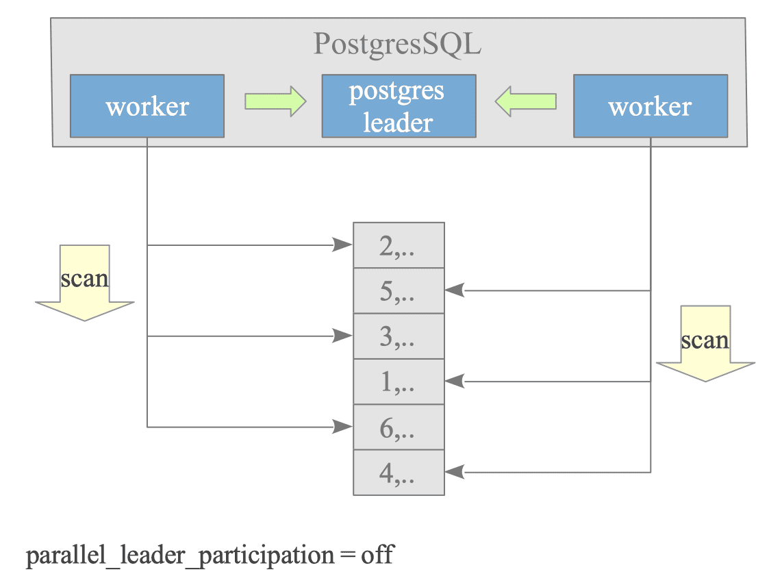
Figure 3.38. Parallel Query Concept.
The parameter parallel_leader_participation, introduced in version 11 (and enabled by default), allows the Leader process to assist in query execution while waiting for responses from Workers. To simplify the following explanations and diagrams, however, the Leader process is assumed to wait only (i.e., parallel_leader_participation is off).
PostgreSQL continues to improve Parallel Query capabilities with each release. Table 3.4 highlights key updates from the official release notes.
| Version | Description |
|---|---|
| 9.6 |
|
| 10 |
|
| 11 |
|
| 12 |
|
| 14 |
|
| 15 |
|
| 16 |
|
- Note: Parallel Query is primarily a read-only feature and currently does not support cursor operations.
The following sections provide an overview of the Parallel Query architecture, followed by an exploration of parallel join operations and parallel aggregation.
3.7.1. Overview
Figure 3.39 illustrates the execution flow of a parallel query in PostgreSQL.
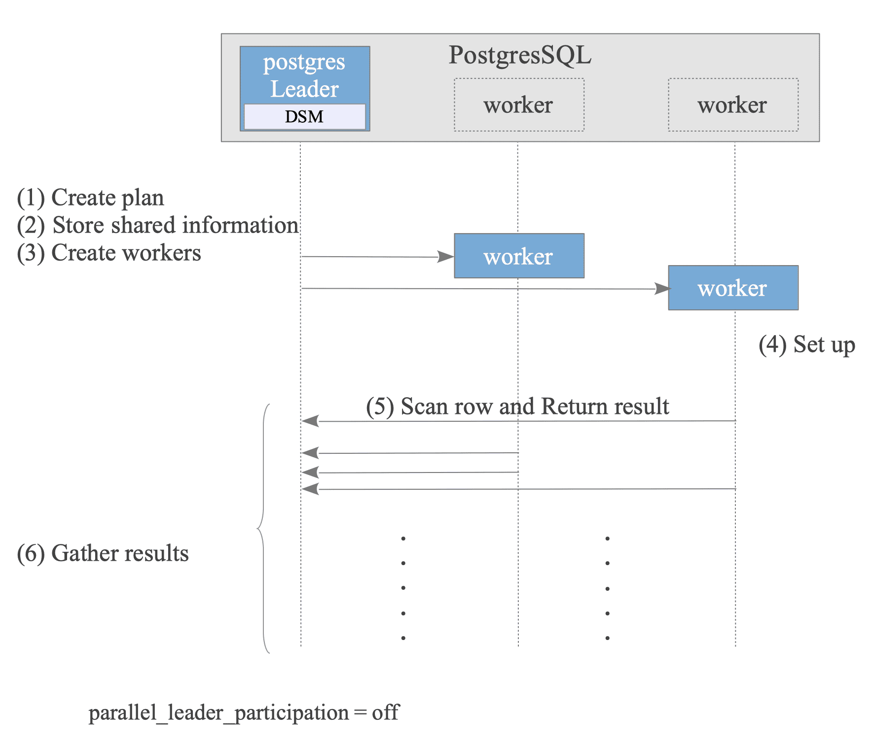
Figure 3.39. How Parallel Query Performs.
-
Leader Creates Plan:
The optimizer creates a plan tree that includes nodes capable of parallel execution. -
Leader Stores Shared Information:
To synchronize execution between the Leader and Worker processes, the Leader stores essential information (such as the plan tree and session state) in its Dynamic Shared Memory (DSM) area. -
Leader Creates Workers:
The Leader starts the background worker processes. -
Worker Sets Up State:
Each worker reads the shared information from the DSM to initialize its internal state, ensuring an execution environment consistent with the Leader. -
Worker Scans and Returns Results:
Each worker actively retrieves and scans data blocks on demand by executing functions such as SeqNext() or IndexNext(). These results are then returned to the Leader. -
Leader Gathers Results:
The Leader receives and aggregates the results from all workers. -
Cleanup:
After the query finishes, the workers are terminated, and the Leader releases the DSM area.
During parallel query processing, the Leader and Worker processes communicate via the DSM area. The Leader process allocates memory space on demand, allowing worker processes to read and write data to these shared regions.
The following concrete examples utilize Table d, created as follows:
testdb=# CREATE TABLE d (id double precision, data int);
CREATE TABLE
testdb=# INSERT INTO d SELECT i::double precision, (random()*1000)::int FROM generate_series(1, 1000000) AS i;
INSERT 0 1000000
testdb=# ANALYZE;
ANALYZE
3.7.1.1. Creating Parallel Plan
The optimizer does not always consider a parallel query. It considers parallel execution only when the size of the table to be scanned is greater than or equal to min_parallel_table_scan_size (default: 8 MB), or if the index size is greater than or equal to min_parallel_index_scan_size (default: 512 kB).
The following is the simplest parallel query plan:
|
|
As shown above, the simplest parallel plan consists of a Gather node and a Parallel SeqScan node.
Figure 3.40 illustrates the plan tree for this query.
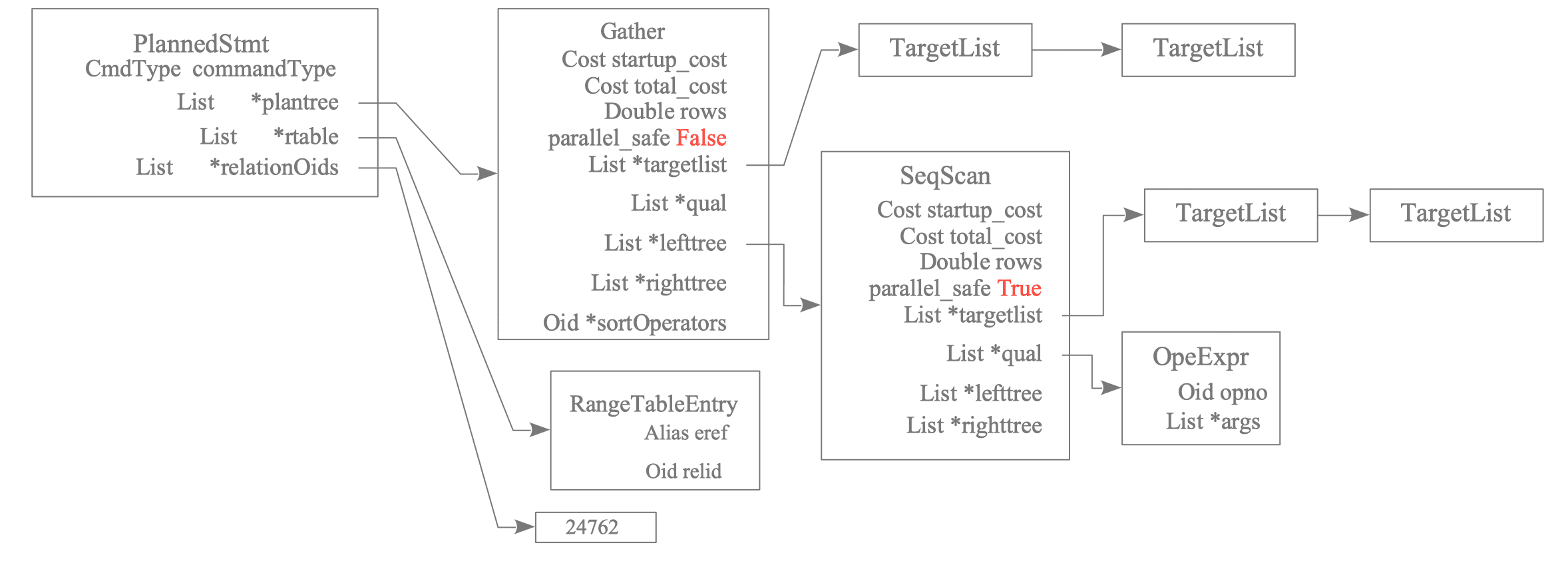
Figure 3.40. Leader's Plan Tree
The Gather node is specific to parallel queries and collects results from the worker processes. In addition to Gather, parallel queries utilize other specialized nodes:
- Gather Merge: Collects results from workers while preserving their sorted order.
- Parallel Append: Used for scanning partitioned tables or UNION ALL queries in parallel (see the Official Documentation).
- Finalize/Partial Aggregate: Used for parallelizing aggregate functions (see Section 3.7.3).
The subplan tree below the Gather node is executed by worker processes.
For a node to be included in this subplan, its ‘parallel_safe’ attribute must be set to True.
In the example above, the Parallel Seq Scan node and its associated filters are executed by the workers.
3.7.1.2. Storing Shared Information
To execute a query collaboratively, the Leader stores information required by the Worker processes in its Dynamic Shared Memory (DSM) area.
The information shared between the Leader and Workers is categorized into two main types: Execution State and Query.
-
Execution State:
This encompasses the environmental information necessary for both the Leader and Workers to execute the same query consistently. (Refer to README.parallel for a comprehensive list). Key components include:- All configuration parameters (GUCs).
- The transaction snapshot and the current subtransaction’s ID (see Chapter 5 for details).
- The set of libraries dynamically loaded via dfmgr.c.
This state is stored by the InitializeParallelDSM() function.
-
Query Information:
This includes data specific to the execution plan and data access methods:- The PlannedStmt and ParamListInfo structures.
- The specialized descriptors for nodes executed by Workers. For example, a Parallel Seq Scan node uses ParallelTableScanDesc, while an Index Scan node uses ParallelIndexScanDesc. Detailed initialization is handled by ExecParallelInitializeDSM().
- Instrumentation and resource usage structures for reporting purposes.
This information is stored by the ExecInitParallelPlan() function.
Additionally, the Leader allocates a TupleQueue (defined in tqueue.c) within the DSM. This queue serves as the communication channel through which the Leader reads the results returned by the Workers.
3.7.1.3. Creating Workers
The number of workers in the query plan may be different from the number of workers actually started. This is because the total number of workers is limited by the max_parallel_workers parameter. Also, there may not be enough worker slots if other parallel queries are running at the same time.
The EXPLAIN ANALYZE command displays both the “Planned” and “Launched” number of Workers, allowing for verification of resource allocation.
testdb=# EXPLAIN ANALYZE SELECT * FROM d WHERE id BETWEEN 1 AND 100;
                                                    QUERY PLAN
------------------------------------------------------------------------------------------------------------------
 Gather  (cost=1000.00..16609.10 rows=1 width=12) (actual time=60.035..60.994 rows=100 loops=1)
   Workers Planned: 2
   Workers Launched: 2
   ->  Parallel Seq Scan on d  (cost=0.00..15609.00 rows=1 width=12) (actual time=31.073..52.248 rows=50 loops=2)
         Filter: ((id >= '1'::double precision) AND (id <= '100'::double precision))
         Rows Removed by Filter: 499950
 Planning Time: 0.265 ms
 Execution Time: 61.012 ms
(8 rows)
3.7.1.4. Setting Up Workers
Upon startup, each Worker reads the shared Execution State and Query information prepared by the Leader in the DSM.
By applying the Execution State, the Worker initializes its environment to match the Leader’s session precisely. This ensures that configuration parameters, transaction snapshots, and loaded libraries are consistent across all processes involved in the query.
To process the query, the Worker reconstructs its own plan tree from the shared PlannedStmt. The ExecSerializePlan() function (and its counterparts) is used to create a sub-plan tree consisting only of parallel_safe nodes—typically the portion of the Leader’s plan tree located beneath the Gather node.
Figure 3.41 illustrates the relationship between the Leader’s plan tree and the plan tree created for the Worker.
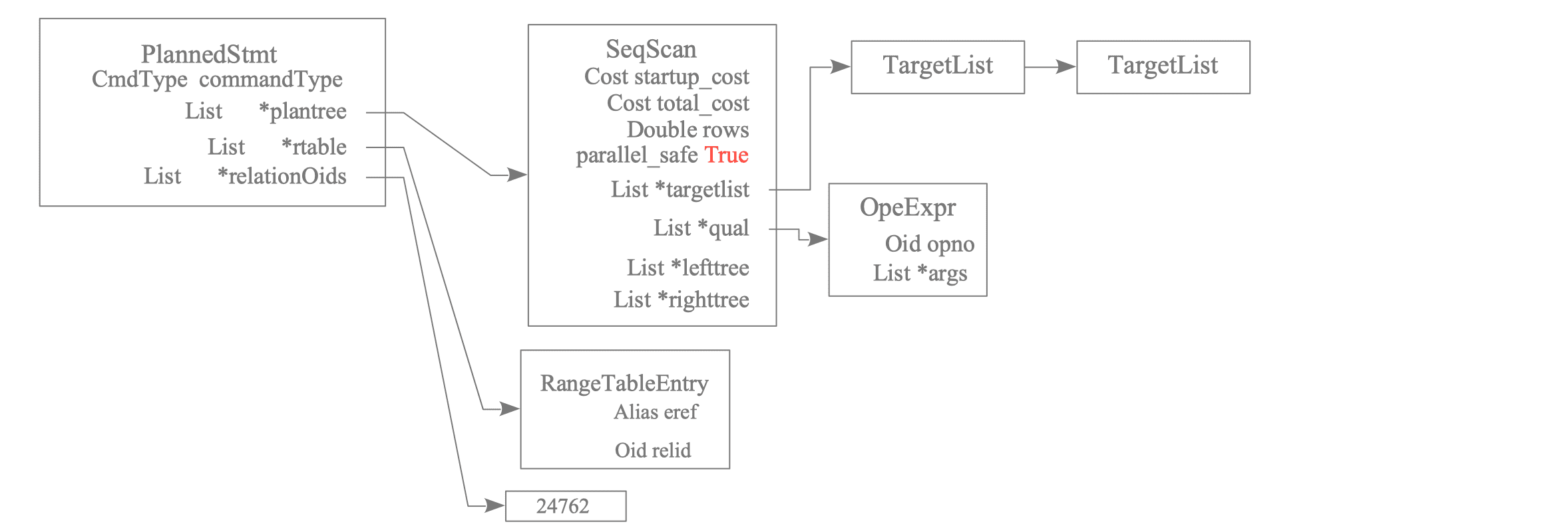
Figure 3.41. Worker's Plan Tree Created from Leader's Plan Tree
3.7.1.5. Scanning Rows and Returning Results
As discussed in Section 3.4.1.1, the executor’s methods for accessing data tuples are highly abstracted. This principle also applies to parallel queries.
Since the Leader and Workers share the query execution environment via the DSM, a single sequential scan can be executed in parallel. Each process actively retrieves and scans data blocks on demand by calling the SeqNext() function.
Similarly, the results are returned to the Gather node via the TupleQueue located in the DSM.
3.7.1.6. Gathering Results
The Gather node is a specific node for parallel queries that collects the results returned by the Workers.
3.7.2. Parallel Join
Parallel queries in PostgreSQL support nested loop joins, merge joins, and hash joins.
The following examples utilize tables d and f.
testdb=# CREATE TABLE d (id double precision, data int);
CREATE TABLE
testdb=# INSERT INTO d SELECT i::double precision, (random()*1000)::int FROM generate_series(1, 1000000) AS i;
INSERT 0 1000000
testdb=# CREATE INDEX d_id_idx ON d (id);
CREATE INDEX
testdb=# CREATE TABLE f (id double precision, data int);
CREATE TABLE
testdb=# INSERT INTO f SELECT i::double precision, (random()*1000)::int FROM generate_series(1, 10000000) AS i;
INSERT 0 10000000
testdb=# \d d
                      Table "public.d"
 Column |       Type       | Collation | Nullable | Default
--------+------------------+-----------+----------+---------
 id     | double precision |           |          |
 data   | integer          |           |          |
Indexes:
    "d_id_idx" btree (id)

testdb=# \d f
                      Table "public.f"
 Column |       Type       | Collation | Nullable | Default
--------+------------------+-----------+----------+---------
 id     | double precision |           |          |
 data   | integer          |           |          |

testdb=# ANALYZE;
ANALYZE
3.7.2.1. Nested Loop Join
In a standard parallel nested loop join, the inner table is not processed in parallel. Instead, each Worker must process the entire inner table independently.
For example, in a materialized nested loop join, each Worker materializes its own copy of the inner table. This redundancy makes the join less efficient as the number of workers increases.
testdb=# SET enable_nestloop = ON;
SET
testdb=# SET enable_mergejoin = OFF;
SET
testdb=# SET enable_hashjoin = OFF;
SET

testdb=# EXPLAIN SELECT * FROM d, f WHERE d.data = f.data AND f.id < 10000;
                                  QUERY PLAN
-------------------------------------------------------------------------------
 Gather  (cost=1000.00..97163469.29 rows=9651513 width=24)
   Workers Planned: 2
   ->  Nested Loop  (cost=0.00..96197317.99 rows=4825756 width=24)
         Join Filter: (d.data = f.data)
         ->  Parallel Seq Scan on f  (cost=0.00..121935.99 rows=4831 width=12)
               Filter: (id < '10000'::double precision)
         ->  Materialize  (cost=0.00..27992.00 rows=1000000 width=12)
               ->  Seq Scan on d  (cost=0.00..18109.00 rows=1000000 width=12)
(8 rows)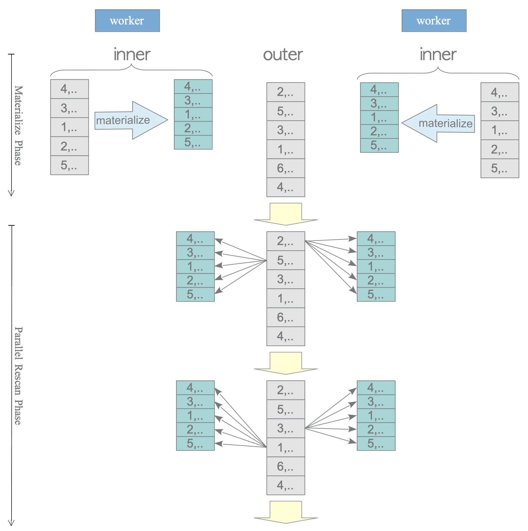
Figure 3.42. Materialize Nested Loop Join in Parallel Query.
In contrast, an Indexed Nested Loop Join is much more efficient. While the inner table scan itself is not “shared,” each Worker uses the index to quickly retrieve only the relevant rows from the inner table.
testdb=# EXPLAIN SELECT * FROM d, f WHERE d.id = f.id AND f.id < 10000;
                                  QUERY PLAN
-------------------------------------------------------------------------------
 Gather  (cost=1000.42..142818.71 rows=967 width=24)
   Workers Planned: 2
   ->  Nested Loop  (cost=0.42..141722.01 rows=484 width=24)
         ->  Parallel Seq Scan on f  (cost=0.00..121935.99 rows=4831 width=12)
               Filter: (id < '10000'::double precision)
         ->  Index Scan using d_id_idx on d  (cost=0.42..4.09 rows=1 width=12)
               Index Cond: (id = f.id)
(7 rows)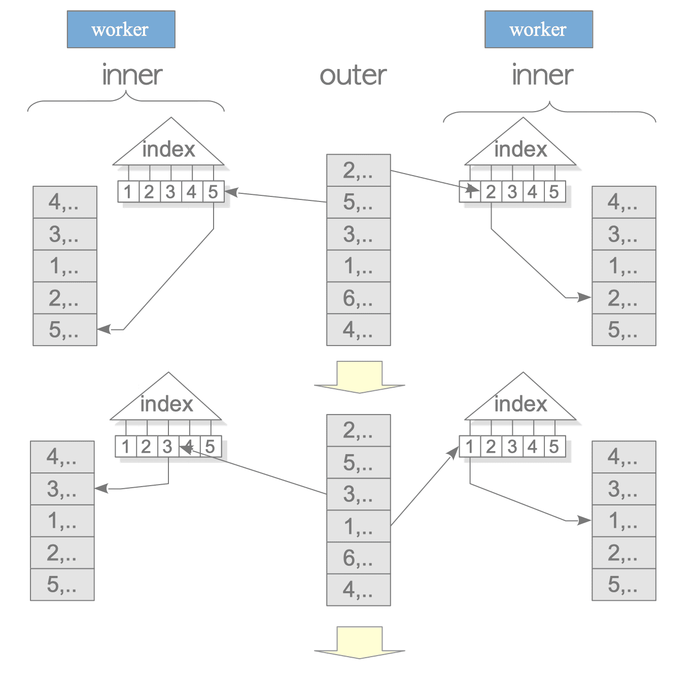
Figure 3.43. Indexed Nested Loop Join in Parallel Query.
3.7.2.2. Merge Join
Similar to nested loop joins, a standard merge join processes the inner table for all rows. Consequently, each Worker must perform its own sorting process for the inner table independently.
However, if the inner table is accessed using an index scan, the join operation can be performed efficiently, similar to an Indexed Nested Loop Join.
testdb=# SET enable_nestloop = OFF;
SET
testdb=# SET enable_mergejoin = ON;
SET
testdb=# SET enable_hashjoin = OFF;
SET
testdb=# EXPLAIN SELECT * FROM d, f WHERE d.id = f.id AND d.id < 100000;
                                       QUERY PLAN
----------------------------------------------------------------------------------------
 Gather  (cost=837387.83..853944.33 rows=97361 width=24)
   Workers Planned: 2
   ->  Merge Join  (cost=836387.83..843208.23 rows=48680 width=24)
         Merge Cond: (f.id = d.id)
         ->  Sort  (cost=836385.61..848880.80 rows=4998079 width=12)
               Sort Key: f.id
               ->  Parallel Seq Scan on f  (cost=0.00..109440.79 rows=4998079 width=12)
         ->  Index Scan using d_id_idx on d  (cost=0.42..3569.24 rows=97361 width=12)
               Index Cond: (id < '100000'::double precision)
(9 rows)
3.7.2.3. Hash Join
In PostgreSQL versions 9.6 and 10, each Worker involved in a parallel hash join builds its own private hash table for the inner table. This leads to high memory usage and redundant work.
testdb=# SET enable_nestloop = OFF;
SET
testdb=# SET enable_mergejoin = OFF;
SET
testdb=# SET enable_hashjoin = ON;
SET
testdb=# SET enable_parallel_hash = OFF;
SET
testdb=# EXPLAIN SELECT * FROM d, f WHERE d.id = f.id;
                                    QUERY PLAN
----------------------------------------------------------------------------------
 Gather  (cost=36492.00..323368.59 rows=1000000 width=24)
   Workers Planned: 2
   ->  Hash Join  (cost=35492.00..222368.59 rows=500000 width=24)
         Hash Cond: (f.id = d.id)
         ->  Parallel Seq Scan on f  (cost=0.00..109440.79 rows=4998079 width=12)
         ->  Hash  (cost=18109.00..18109.00 rows=1000000 width=12)
               ->  Seq Scan on d  (cost=0.00..18109.00 rows=1000000 width=12)
(7 rows)
Parallel Hash Join was introduced in version 11 (controlled by the enable_parallel_hash parameter, which is on by default). With this feature, all Workers cooperate to build a shared hash table in the DSM. This allows for a more efficient build phase and reduces memory overhead.
testdb=# SET enable_parallel_hash = ON;
SET
testdb=# EXPLAIN SELECT * FROM d, f WHERE d.id = f.id;
                                      QUERY PLAN
--------------------------------------------------------------------------------------
 Gather  (cost=22801.00..304736.59 rows=1000000 width=24)
   Workers Planned: 2
   ->  Parallel Hash Join  (cost=21801.00..203736.59 rows=500000 width=24)
         Hash Cond: (f.id = d.id)
         ->  Parallel Seq Scan on f  (cost=0.00..109440.79 rows=4998079 width=12)
         ->  Parallel Hash  (cost=13109.00..13109.00 rows=500000 width=12)
               ->  Parallel Seq Scan on d  (cost=0.00..13109.00 rows=500000 width=12)
(7 rows)
3.7.3. Parallel Aggregate
Most aggregate functions in PostgreSQL can be processed in parallel.
Whether a specific function supports parallelization depends on whether its Partial Mode is set to YES in the Official Documentation.
The planner chooses between two primary strategies based on the estimated number of target rows.
3.7.3.1. Strategy 1: Simple Aggregation (Small Row Count)
When the predicted number of rows is small, workers perform the scan, but the actual aggregation happens in the Leader process:
- Each Worker scans rows via a Parallel Seq Scan node.
- The Gather node receives these raw rows from the Workers.
- The Aggregate node calculates the final result from the gathered rows.
testdb=# EXPLAIN SELECT avg(id) FROM d where id BETWEEN 1 AND 10;
                                        QUERY PLAN
------------------------------------------------------------------------------------------
 Aggregate  (cost=16609.10..16609.11 rows=1 width=8)
   ->  Gather  (cost=1000.00..16609.10 rows=1 width=8)
         Workers Planned: 2
         ->  Parallel Seq Scan on d  (cost=0.00..15609.00 rows=1 width=8)
               Filter: ((id >= '1'::double precision) AND (id <= '10'::double precision))
(5 rows)

testdb=# EXPLAIN SELECT var_pop(id) FROM d where id BETWEEN 1 AND 10;
                                        QUERY PLAN
------------------------------------------------------------------------------------------
 Aggregate  (cost=16609.10..16609.11 rows=1 width=8)
   ->  Gather  (cost=1000.00..16609.10 rows=1 width=8)
         Workers Planned: 2
         ->  Parallel Seq Scan on d  (cost=0.00..15609.00 rows=1 width=8)
               Filter: ((id >= '1'::double precision) AND (id <= '10'::double precision))
(5 rows)
3.7.3.2. Strategy 2: Partial/Finalize Aggregation (Large Row Count)
When the predicted number of rows is large, it is more efficient to reduce the data volume before sending it over the DSM:
- Each Worker performs a Partial Aggregate on its locally scanned rows.
- The Gather node collects these intermediate, partially aggregated results (rather than raw rows).
- The Finalize Aggregate node combines the intermediate results into a final answer.
testdb=# EXPLAIN SELECT avg(id) FROM d where data > 100;
                                     QUERY PLAN
-------------------------------------------------------------------------------------
 Finalize Aggregate  (cost=16485.14..16485.15 rows=1 width=8)
   ->  Gather  (cost=16484.93..16485.14 rows=2 width=32)
         Workers Planned: 2
         ->  Partial Aggregate  (cost=15484.93..15484.94 rows=1 width=32)
               ->  Parallel Seq Scan on d  (cost=0.00..14359.00 rows=450371 width=8)
                     Filter: (data > 100)
(6 rows)

testdb=# EXPLAIN  SELECT var_pop(id) FROM d where data > 100;
                                     QUERY PLAN
-------------------------------------------------------------------------------------
 Finalize Aggregate  (cost=16485.14..16485.15 rows=1 width=8)
   ->  Gather  (cost=16484.93..16485.14 rows=2 width=32)
         Workers Planned: 2
         ->  Partial Aggregate  (cost=15484.93..15484.94 rows=1 width=32)
               ->  Parallel Seq Scan on d  (cost=0.00..14359.00 rows=450371 width=8)
                     Filter: (data > 100)
(6 rows)
3.7.3.3. Mathematical Logic for Parallel Aggregation
To combine results from different workers (e.g., sums, averages, and variances), PostgreSQL uses the following formulas:
$$ \begin{align} S_{n} &= S_{n_{1}} + S_{n_{2}} \\ A_{n} &= \frac{1}{n_{1} + n_{2}} (S_{n_{1}} + S_{n_{2}} ) \\ V_{n} &= (V_{n_{1}} + V_{n_{2}}) + \frac{n_{1} n_{2}}{n_{1} + n_{2}} \left(\frac{S_{n_{1}}}{n_{1}} - \frac{S_{n_{2}}}{n_{2}} \right)^{2} \end{align} $$The Finalize Aggregate node uses these formulas to merge the partial results. For queries involving three or more workers, this process is repeated iteratively to reach the final value.
Given:
- A dataset: $ \{ x_{i} | 1 \le i \le n = n_{1} + n_{2} \} $
- The overall average: $A_{n} = \sum_{i=1}^{n_{1}+n_{2}} x_{i}$
- The sum of the first part of the dataset: $S_{n_{1}} = \sum_{i=1}^{n_{1}} x_{i}$
- The variance of the first part: $V_{n_{1}} = \sum_{i=1}^{n_{1}} (x_{i} - \frac{S_{n_{1}}}{n_{1}})^{2}$
- The sum of the second part of the dataset: $S_{n_{2}} = \sum_{i=1+n_{1}}^{n_{1}+n_{2}} x_{i}$
- The variance of the second part: $V_{n_{2}} = \sum_{i=1+n_{1}}^{n_{1}+n_{2}} (x_{i} - \frac{S_{n_{2}}}{n_{2}})^{2}$
To Prove:
The variance of the entire dataset, $V_{n}$, can be expressed in terms of $V_{n_{1}}$, $V_{n_{2}}$, $S_{n_{1}}$, and $S_{n_{2}}$ as follows:
$$ V_{n} = V_{n_{1}} + V_{n_{2}} + \frac{n_{1} n_{2}}{n_{1} + n_{2}} \left( \frac{S_{n_{1}}}{n_{1}} - \frac{S_{n_{2}}}{n_{2}} \right)^{2} $$